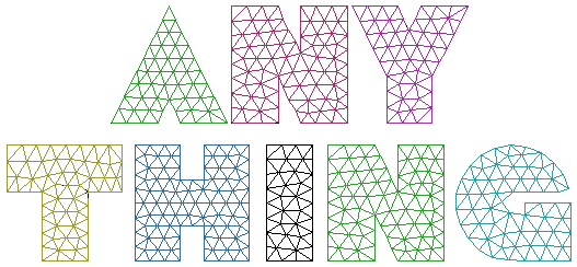
 In the finite-element method, a distributed
physical system to be analysed is divided into a number (often large)
of discrete elements.
In the finite-element method, a distributed
physical system to be analysed is divided into a number (often large)
of discrete elements.
W. Robert J. Funnell
Dept. BioMedical Engineering, McGill University
This is a very brief introduction to some of the concepts involved in the finite-element method. For more details, many text books are available (e.g., Fundamentals of the Finite Element Method, H. Grandin Jr., Macmillan, New York, xvi + 528 pp, 1986).
In the finite-element method, a distributed
physical system to be analysed is divided into a number (often large)
of discrete elements.
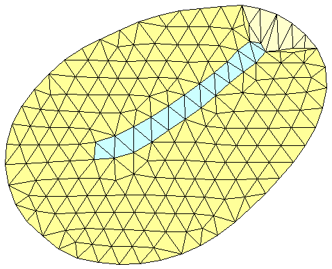
The complete system may be complex and irregularly shaped, but
the individual elements are easy to analyse.
The
division into elements may partly correspond to natural subdivisions
of the structure. For example, the eardrum may be divided into groups
of elements corresponding to different material properties.
Most or all of the model parameters have very direct relationships to the structure and material properties of the system.
A finite-element model generally has relatively few free
parameters whose values need to be adjusted to fit the data. This assumes,
of course, that the parameters are known a priori from other
measurements.
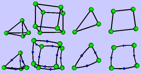
The elements
The elements may model mechanics, acoustics, thermal fields,
electromagnetic fields, etc., or coupled problems.
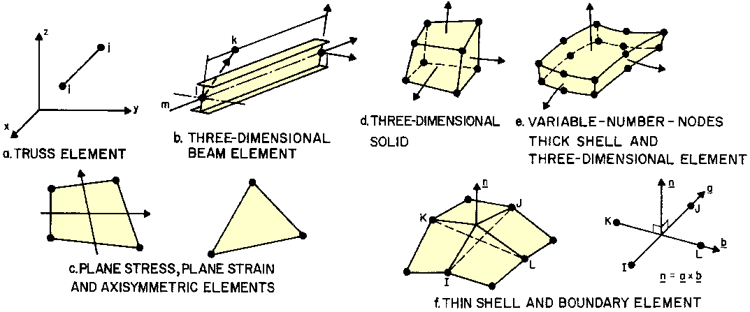
In a mechanical problem, the elements may model membranes,
beams, thin plates, thick plates, solids, fluids, etc.
The behaviour of a particular type of element is analysed in terms of the loads and responses at discrete nodes. This analysis is often based on the Rayleigh-Ritz procedure, which is discussed in Section 2.
An example of a particularly simple element formulation is
presented in Section 3.
The result of the analysis of a typical element type is a small matrix relating a vector of nodal displacements to a vector of applied nodal forces.
The components of the matrix can be expressed as functions of the shape and properties of the element, and the values of the components for a particular element can then be obtained by substituting the appropriate shape and property parameter values into the formulæ.
Once the element matrices have been calculated, they are all combined together into one large matrix representing the whole complex system, as discussed in Section 4.
This procedure was introduced by Ritz in 1908 and is a generalization of a technique used by Rayleigh in 1877. It is the most common procedure used for formulating finite-element approximations. The following discussion is based on Stakgold (1968, pp. 332-335).
| A functional is a function of a function. |
| An admissible function is one which satisfies the boundary conditions, as well as certain continuity conditions. |
The procedure is based on the theorem of minimum potential energy in mechanics: if one has a functional giving the potential energy of a system, then the ‘admissible’ function which minimizes that functional is the solution of the system.
In practice it will be difficult or impossible to find, among all admissible functions, the one which minimizes the functional. Thus, we must limit the set of functions over which we shall attempt to minimize the functional.
| The convention here is that bold lowercase variables represent vectors, and bold uppercase variables represent matrices. |
The Rayleigh-Ritz procedure consists of restricting the search to a particularly simple subset of admissible functions, namely, the space of linear combinations of \(n\) independent admissible basis functions \(w_i(\mathbf{x}), i=1,2,...n\).
The \(w_i\) represent, for example, displacement fields for a mechanical problem, and are functions of the spatial coördinates \(\mathbf{x}\).
The value of \(n\) is chosen to be as small as is consistent with the accuracy required of the answer. The particular set of basis functions used is more or less arbitrary, as long as they are independent and admissible.
Examples of independent basis functions?
The linear combinations can be expressed as
|
| (Eqn. 1) |
Since each of the basis functions is admissible, every function in the space of linear combinations will also be admissible.
Recall that we wish to find the \(w(\mathbf{x})\) which minimizes the energy functional \(F(w)\).
Since , is now a function of the .
Minimizing \(F(w)\) over the set of linear combinations of the basis functions corresponds to choosing the \(c_i\) such that \(F\) is minimal. Thus, we take the partial derivative of \(F\) with respect to each \(c_i\) in turn and set it to zero.
We end up with a set of \(n\) algebraic equations in \(c_i\):
| (Eqn. 2) |
Thus, the boundary-value problem for a single element has been reduced to the solution of \(n\) linear algebraic equations in \(n\)unknowns.
Equivalently, it has been reduced to a matrix equation with an \(n \times n\) matrix.
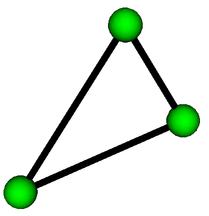
If the element is a triangle, and each vertex has 1 degree of freedom, then the matrix will be 3×3. If each vertex has 3 degrees of freedom (\(x\), \(y\) and \(z\) displacement components) then the matrix will be 9×9.
As an example of the type of analysis involved in the formulation
of finite elements, we shall consider the analysis of a very simple
case: a plane vibrating membrane which we shall divide into triangular
elements which use only three basis functions.

The differential equation governing a plane membrane under tension and
vibrating sinusoidally (Rayleigh, 1877) is
| (Eqn. 3) |
If we define
\(\lambda^2 = \sigma \omega^2 / T\) and \(g = p/T\),
then it can be shown (Forsythe & Wasow, 1960,
Chap. 3) that the energy functional corresponding to this system is
| (Eqn. 4) |
The three integral terms on the right-hand side represent energy due to membrane tension, inertia, and the applied pressure, respectively.
This functional is the one to be minimized using the Rayleigh-Ritz procedure.
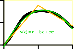
As for what basis functions to use, the simplest choice is a set which permits the displacement field over the element to be a general linear function of \(x\) and \(y\). For this, three basis functions are needed.
There are two ways of formulating them, one based on Cartesian coördinates and the other on so-called ‘natural’ coördinates. The ultimate result is the same, but in some circumstances one of the two formulations may be superior.
The Cartesian-coördinate method
involves choosing as basis
functions the set \(\{1, x, y\}\).
The displacement at any
point \((x, y)\) in the element is then given by a linear
combination of these three functions, namely,
| (Eqn. 5) |
Applying this equation at each of the three vertices of the element,
we obtain
| (Eqn. 6) |
| (Eqn. 7) |
Following the Rayleigh-Ritz procedure, we substitute for \(w\)
using equation 5 in equation 4, carry out the double integrations,
and differentiate with respect to each of the \(c_i\)
in turn. Setting the derivatives equal to zero then results in a set
of algebraic equations for the \(c_i\):
| (Eqn. 8) |
The components of the matrices \(\mathbf{A}\) and \(\mathbf{B}\) are functions of \(\lambda\) (which depends on the frequency, tension and area density) and of the vertex coördinates of the triangular element.
This equation is the one that would have to be solved if the
element were alone. If it is part of a larger system, however, the
equation must be transformed so that it can be combined with similar
equations representing other elements. We do this by expressing it in
terms of the nodal displacements \(w_i\) rather than
the \(c_i\), by using equation 7
.
The algebraic
equations describing the behaviour of the element now become
| (Eqn. 9) |
| (Eqn. 10) |
The right-hand side is a vector of nodal applied forces and \(\mathbf S\) is known as the element stiffness matrix.
For a triangle with one degree of freedom at each node, the stiffness matrix will be 3×3. Each component of the matrix represents the stiffness existing between one node and another (or itself, along the diagonal). The stiffness relationship between two nodes is symmetrical.
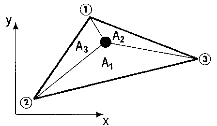 The natural-coördinate method (Desai & Abel, 1972,
pp. 88-91) expresses the location of any point in the triangular
element by the area coördinates
\((\zeta_1, \zeta_2, \zeta_3)\),
where
\(\zeta_i = A_i / A\); \(A\) is the total area of the
triangle and the \(A_i\) are as shown in the
Figure. (Note that the three \(\zeta_i\) are not
independent, since they add up to 1.) We can use the \(\zeta_i\)
as the set of basis functions. It can be shown
that in this case the coefficients \(c_i\) become the
nodal displacements \(w_i\).
Following the
Rayleigh-Ritz procedure again leads to equation 10.
The natural-coördinate method (Desai & Abel, 1972,
pp. 88-91) expresses the location of any point in the triangular
element by the area coördinates
\((\zeta_1, \zeta_2, \zeta_3)\),
where
\(\zeta_i = A_i / A\); \(A\) is the total area of the
triangle and the \(A_i\) are as shown in the
Figure. (Note that the three \(\zeta_i\) are not
independent, since they add up to 1.) We can use the \(\zeta_i\)
as the set of basis functions. It can be shown
that in this case the coefficients \(c_i\) become the
nodal displacements \(w_i\).
Following the
Rayleigh-Ritz procedure again leads to equation 10.
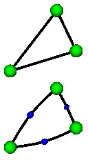
Additional nodes on edges and possibly in interior
Advantage of higher order
Since the behaviour of each element has been described in terms of its behaviour at its edges, and in fact at certain discrete nodes along its edges, the assembly of element matrices into a system matrix is simply an expression of
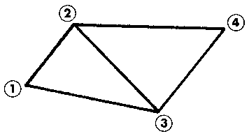 Suppose that a system to be studied consists of two triangular
elements interconnected as shown in the Figure. Suppose that
substituting the vertex coördinates and material properties into the
formulæ obtained from the mechanical analysis gives components
\(a_{ij}\) for the element stiffness matrix for the first element, and
\(b_{ij}\) for the second element. Then equation 10 yields
Suppose that a system to be studied consists of two triangular
elements interconnected as shown in the Figure. Suppose that
substituting the vertex coördinates and material properties into the
formulæ obtained from the mechanical analysis gives components
\(a_{ij}\) for the element stiffness matrix for the first element, and
\(b_{ij}\) for the second element. Then equation 10 yields
| and | (Eqn. 11) |
Now, since the \(w_2\) and \(w_3\) in
Equation 11 are the same for both elements, we can combine the two
equations as follows:
| (Eqn. 12) |
The system boundary conditions now consist of prescribed values for
some of the \(w_i\). One way to handle these
constrained \(w_i\) is to remove them from the vector
of unknowns – with appropriate node numbering,
\(\mathbf w\) can be partitioned into two parts, the
unknown displacements \(\mathbf w _1\) and the
prescribed values \(\mathbf w _2\). Partitioning
\(\mathbf S\) and \(\mathbf f\) correspondingly, we obtain
| (Eqn. 13) |
| (Eqn. 14) |
The system to be solved is now smaller.
Any extra forces applied to individual nodes can also be added into the right-hand side. The equation then represents the entire boundary-value problem, and is solved using one of a variety of techniques, such as Gauss-Jordan elimination.
 \[ \mathbf K \mathbf u = \mathbf f \]
In this case there are no inertial or damping effects, or at least they are negligible. In the middle ear, for example, a static solution is applicable up to about 300 Hz.
At very low frequencies the ‘static’ solution
may no longer work because of very slow time-varying effects such as
thermal drift in electrical circuits, and creep or relaxation in
biomechanical systems.
If we consider harmonic vibrations, \(\mathbf M \ddot {\mathbf u}\) becomes \(- \omega^2 \mathbf M \mathbf u\). Because of the lack of damping (or energy dissipation), forcing functions at certain frequencies will lead to infinite displacements, so we consider the unforced problem: \[\mathbf K \mathbf u - \omega^2 \mathbf M \mathbf u = 0\]
Equivalently, \[\mathbf K \mathbf u = \omega^2 \mathbf M \mathbf u\]
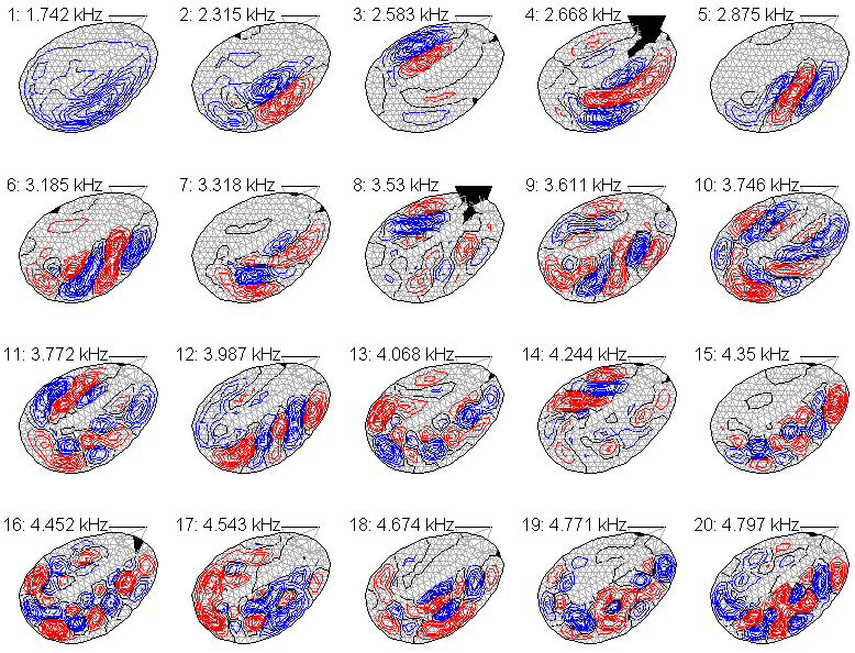
This is a generalized eigenvalue/eigenvector problem.
The eigenvalues of
\(\mathbf K \mathbf u = \omega^2 \mathbf M \mathbf u\)
correspond to the squares of the natural frequencies,
and the eigenvectors correspond to the associated modes of vibration.
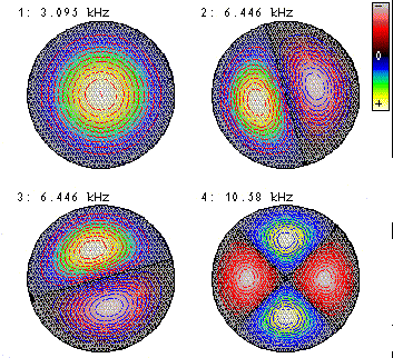
Note the two degenerate modes at 6.446 kHz.
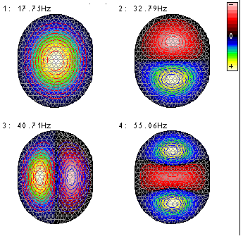 Removing the circular symmetry removes the degenerate modes.
There are multiple approaches to solving this problem.
Modal analysis involves representing responses to
arbitrary inputs by weighted superposition of a number of the natural
modes. This is very efficient if a small number of modes can be used
without losing accuracy.
Modal analysis is not very useful for many biological systems,
where the asymmetries and irregularities lead to large numbers of
closely spaced natural frequencies.
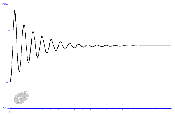
An alternative approach is to use direct time-domain integration. \[ \mathbf K \mathbf u + \mathbf C \dot {\mathbf u} + \mathbf M \ddot{\mathbf u} = \mathbf f \]
For example: step response.
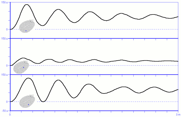
Different time courses at different locations in model.

Can differentiate step response to get impulse response.
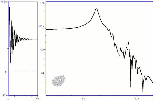
Or take Fourier Transform to get frequency response.
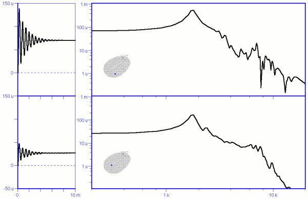
Different frequency responses at different locations.
For harmonic vibrations, the equation becomes
\[\mathbf K \mathbf u + j \omega \mathbf C \mathbf u - \omega^2 \mathbf M \mathbf u = \mathbf f\]
so for a given frequency it has the same form as the static case but with a
complex-valued system matrix:
\[( \mathbf K + j \omega \mathbf C - \omega^2 \mathbf M ) \mathbf u = \mathbf f .\]
R. Funnell Last modified: 2025-05-29 10:11:54