Fad: Finite-element preprocessor

Installation Usage Use with Gmsh

Fad is a programme for manipulating 3-D finite-element models. It takes .sap plain-text model-definition files as input.

Fad is implemented in Fortran. It was originally developed under VMS, and is currently being developed under Compaq (Digital) Unix for Alpha; GNU/Linux for Alpha and Intel; and (alas) Microsoft Windows. The binary is available for Unix and GNU/Linux by request; the binary for Windows is offered here. It can be used for any purpose as long as I am informed of its use. So far there is no documentation beyond the very incomplete beginning that you're looking at.

In this documentation, square brackets [ ] are used to indicate optional command arguments and should not be included in the commands themselves. The visible-space character ␣ is sometimes used to emphasize where space characters should be used in commands.

In prompts within Fad, square brackets are sometimes used to indicate default values, that is, values that will be used if you just type Enter.

1. Installation

1.1 Installation under GNU/Linux

Download the Fad executable from here and do chmod u+x fad to make it executable.

• amd64 binary (x86_64)
• ia32 binary (i386) (out of date; ask me)

(If your computer is part of the McGill BME network, you can create a symbolic link (ln -s) to the executable on probeShare, in order to always run the latest version.)

Make sure that the xdg-utils package has been installed (e.g., by doing sudo apt-get install xdg-utils). (It is used to open Fad's documentation with the default Web browser.) Follow the general instructions for installation of Dip software.

You can run Fad by opening a terminal window, cd’ing into the directory where you saved it and giving the command ./fad, or by giving the command ./Downloads/fad (assuming that you saved Fad in the Downloads subdirectory of your home directory. Do not include & at the end of the fad command.

Fad requires at least about 1500 to 2000 MB of memory to run. If Fad fails to run, check that you have enough free memory. (If running under VirtualBox, try increasing the amount of memory allocated to your virtual machine.)

1.2 Installation under MS Windows 95/98/NT/2000/XP/Vista

A version for MS Windows is not currently available.

2. Usage

2.1 Starting Fad

When Fad is run, it should display a Plotting to? question. Normally you should just type Enter (or Return) here. You should then see a Do (? for help) ? prompt. After every action you should be returned to this prompt. If not, it means that Fad has crashed and you should look for an error message.

Typing ? and Enter will invoke your default Web browser to display this page of documentation. Typing ? as a second character for any command, and in some other places in Fad, will cause the same documentation page to be displayed, sometimes positioned at the relevant topic. Displaying this on-line help requires that you have an Internet connection open.

The first command that you give would normally be R to read in a .sap file, or perhaps I to import a file that is in some other format, or G to generate a new model. The commands are not case-sensitive, so you could equally well use r, i and g.

Fad attempts to create a log file called fad_log.tmp in your home directory. If that is successful, then various parts of Fad may record things there.

2.2 Read

When you give the R command you will be presented with a list of recently opened files. Select one of them by clicking, or click on + Other to browse and find another file. See also further information about using Dip file menus.

After a model has been read in, Fad automatically displays it and also displays some numbers at the bottom of the window:

• If the model includes shell elements (type 6) then numbers of edges are displayed: reversed, surface, boundary, interior and duplicate. (It claims to also display the total number of edges but currently it’s just set to zero.) See Use with Gmsh for information about how to interpret the numbers.
• If the model includes solid elements (types 5, 8 and 13) then numbers of faces are displayed (surface, boundary, interior, duplicate and total) and numbers of nodes are displayed (surface, non-surface and total).

Sometimes it’s desirable to read in two models at the same time. To read in both a primary model and a secondary model, use the command R␣/sec. When presented with the file-selection menu, open the secondary file first and then the primary file. The Align and Join commands are based on the use of secondary models; the Plot command includes various ways of controlling how they're displayed together with the primary model; and the Modify and Import commands make use of them.

2.3 Write

This command writes out the current primary model in .sap format. The secondary model, if any, is not included; if you want it to be included, use the Join command before the Write command. Any current rotations are not applied; if you want them to be applied, use the Fix command before the Write command.

2.4 Plot

2.4.1 Introduction

The simplest plot command is P (or p), which will plot every edge of every element and then activate interactive rotation, translation and clipping.

Many options are available for the Plot command. For example, the command

2.4.2 Interactive rotation, translation and clipping

Once you have used the P command to display (plot) a model (and the secondary model if there is one), an interactive rotation, translation and clipping tool will appear in the bottom left corner. Rotations and translations are reflected immediately when the model is plotted, but are not applied to the actual model coördinates until and unless the Fix command is given.

The x, y and z axes are displayed in red, green and blue, respectively. Below the axes is a concise indication of the current status of the tool. In the examples shown on the right, for example:

• R indicates that the tools are in rotation mode, which is the initial mode. The other two modes are translation and clipping. To the left of the model(s) are displayed the current orientation(s), the current translation(s) if non-zero, and the current clipping value if active.
• X and Y indicate the currently active axis, which can be either X, Y or Z.
• W indicates that the tools are in the world-coördinates mode, as opposed to the object-coördinates mode.
• 10 and 5 indicate the current incremental values for changing the rotation, translation or clipping plane. The initial setting is 10°.
• (i) indicates that the tools are in the Immediate mode.
• The second example on the right shows what the tool might look like when a secondary model has been read in together with the primary model. The B indicates that interactive changes will be applied to both the primary and secondary models, rather than just one or the other. The x, y and z axes for the secondary model are displayed in lighter shades of red, blue and green.

Typing just Enter causes the currently specified action to be taken, either rotating or translating the model or changing the position of the clipping plane. Typing a number followed by Enter will change the rotation, translation or clipping step size. Typing a letter followed by Enter changes other settings of the tool. The following commands are available:

• Typing Q or CtrlZ returns to the Fad prompt.
• Typing X, Y or Z will change the active axis.
• The A command followed by three numbers will specify an absolute rotational (or translational) position. For example, A␣0,0,0 (or just A) will reset the model to its initial position.
• If a secondary model has been read in, P causes actions to be applied only to the primary model; S causes them to be applied only to the secondary model; and B causes them to be applied to both models.
• Normally the rotations are applied about the World coördinate axes, fixed in space. The O command will cause the rotations to be applied about the coördinate axes fixed in the object. The W command will cause the tool to revert to using the world coördinate axes.
• The T command causes the tool to perform translations rather than rotations. Unless you’re displaying a secondary model as well as the primary model, translation doesn’t have a visual effect because the display is automatically centred.
• The C command causes the tool to adjust the z-clipping. This only has an effect if the /clip option was used with the plot command.
• The I command will toggle between Immediate mode and not-Immediate mode. In not-Immediate mode, the actual model won't be replotted until the P command is given. This may be useful for slow computers or large models for which the replotting takes a long time.
• The ~ command causes the current rotation or translation increment value to be multiplied by −1. This command can also be given using the character `, that is, the unshifted version of ~ on many keyboards, thus making it unnecessary to use the Shift key.

There is no zoom function as part of the plot command. By default the model is automatically zoomed to almost fill the display area. This automatic scaling is based on which elements are selected in the primary model; if all elements are selected then the scaling is based on all of the nodes in the model, which may yield a different result from scaling based on all of the elements if there are some nodes that are not used in any element. If a secondary model is also displayed, then the scaling will also take into account all of its nodes (since element selection is not yet implemented for the secondary model). Something equivalent to zooming can be obtained using the Modify window command.

2.4.3 Plotting levels

The first parameter of a plot command is a plotting level from 0 to 9. If no plotting level is specified, it is taken to be 1.

A plotting-level value of 0 (zero) for the plot command causes only the nodes to be plotted, without elements.

If the plotting-level value is greater than 0, it specifies the minimum desired plotting level for which element edges will be plotted, with higher numbers corresponding to more important edges:

• 1: every edge including duplicates – when 2 elements share an edge, the edge will be plotted twice, once for each element
• 3: every edge except duplicates – this may be faster, but may be misleading when plotting subsets of the elements in a model, since some edges may not be displayed
• 5: edges between different material types
• 7: edges on the outsides of objects
• 8: edges of element faces that have pressure applied to them (for tetrahedral elements only)
• 9: duplicate edges that are not reversed with respect to each other (for shell elements only; probably indicates reversed elements or superimposed elements)

An important use of plotting levels is to confirm that a 3-D surface is simple and closed and has all of its triangles oriented in the correct direction, in which case a p␣5 command should display nothing at all. This condition must be satisfied before using Fad with Gmsh to create a tetrahedral mesh.

A quadrilateral element face is plotted as two triangles, which are formed by using an arbitrarily selected diagonal. That diagonal effectively has a plotting level less than 1 and is never plotted.

2.4.4 Which nodes or elements to plot

If elements are being plotted (plotting level ≥ 1), the plotting level may be followed by S, which means that elements will be plotted for the secondary model, and then by the element type (see Select). If no element type is specified, all elements are considered.

After the plotting level (or the element type if applicable) three optional values can be given: istart, istop and istep.
If none of them is specified, all of the nodes (or elements) will be plotted.
If istart is specified but istop is not, istop will be set = istart and a single node (or element) will be plotted.
If istep is not specified, it is taken to be 1.

As examples:
p␣3␣6␣20 will plot just type-6 (shell) element number 20
p␣0␣50␣100 will plot every node from 50 to 100
p␣5␣6␣1␣100␣2 will plot level-5 edges for every second type-6 element from 1 to 100.

The elements to be plotted can also be controlled using the Select command.

2.4.5 Options

The table on the right summarizes the available options for the plot command. The sections below give further information about some of the options.

2.4.5.1 /coord – Node coördinates

This option displays the x, y and z coördinates for the last node plotted. (Although this information is actually displayed for every node, it is subsequently overwritten for all but the last node.)

2.4.5.2 /usage – Node usage

This option analyzes which elements each node is used in. Each node is displayed with a green symbol whose size is proportional (up to a maximum) to how many elements the node is used in. If a node is unused (i.e., not used in any elements, or ‘orphan’) then it is displayed with a red symbol. For the last node displayed, a list is displayed of which elements the node is used in. (Although this information is actually displayed for every node, it is subsequently overwritten for all but the last node.) A message is also displayed that specifies which node has the greatest usage, and what that usage is.

2.4.5.3 /near – Nearness to other nodes

This option provides an analysis of how close together nodes are, including both primary and secondary models. It is good for identifying duplicate nodes, and nodes that are so close together that they probably should be considered as duplicates.

For each node the distance to its nearest neighbour is calculated. If there are any duplicate (i.e., exactly superimposed nodes, with identical coördinates) a message will be displayed saying how many there are. Then a message will be displayed giving the ratio of the smallest to the largest nearest-neighbour distances. If this ratio is greater than, say, 100, it means that some nodes are much more closely spaced than others.

Duplicate nodes are displayed as red diamonds (or orange for the secondary model). Nodes that have almost the maximum nearest-neighbour distance are displayed as large black triangles (or blue for the secondary model). The remaining nodes are displayed as squares, with the symbol sizes larger for smaller nearest-neighbour distances, and with colours ranging from black to red (or from blue to orange for the secondary model).

2.4.5.4 /size – Symbol size for nodes

Nodes are plotted as squares. This size parameter specifies the size of the squares, from zero to an enforced maximum value of 20. The default size is 2. (The size of the square for a given size parameter depends on the screen resolution.) If the size parameter = 0, each node is plotted as a single dot. If this option is used when displaying elements then the nodes will also be plotted. (This currently doesn't work when z buffering is used.)

2.4.5.5 /fill – Filled triangles

By default the model is plotted as a wireframe. The /fill causes each triangle to be filled with a colour specified in the model-definition file, either explicitly or implicitly (e.g., based on material type). Triangles whose nodes are numbered counterclockwise as seen by the user are considered to be facing the user, and triangles that face away from the user are displayed as orange. If a surface is closed and all of its triangles are correctly oriented then no orange triangles should appear. (Faint orange lines may appear as artefacts.)

2.4.5.6 /-zbuffer – Do not use z-buffer algorithm

By default, Fad plots filled triangles using a relatively fast z-buffer algorithm. The /-zbuffer option causes Fad to use a slower method: Fad sorts the triangles and then displays them from back to front. Normally a small green circle should appear above the Plot interaction tool. A red cross appears if the sorting algorithm fails, usually because of intersecting triangles. In this case some triangles will be dropped, creating a hole, and therefore orange triangles may appear even though they are correctly oriented. The fact that a green circle appears does not guarantee that there are no intersecting triangles.

2.4.5.7 /unselected – Plot unselected elements

Elements that have been unselected are plotted anyways, but with grey instead of their usual colour.

2.4.5.8 /volume – Element volume

The volumes of tetrahedral elements are calculated and the range is displayed. If used with /fill, the colour of any tetrahedron with a negative or zero volume is changed to deep pink.

2.4.5.9 /rot2 – Secondary model

By default, rotations and translations are applied to both the primary model and the secondary model if there is one. Use the /-rot2 qualifier on the plot command to cause the rotations and translations not to be applied to the secondary model.

2.5 Import

Fad can import (with restrictions in some cases) the following formats:

• GRUMMP volume mesh (.vmesh) and an old Fad variant (.vmesh_fad)
• GRUMMP 3-D geometry file (.bdry)
• Sap results file (.res)
• GiD tetrahedral mesh (.msh)
• Gmsh tetrahedral mesh (.msh); Fad can distinguish between GiD and Gmsh .msh files, and can distinguish between Gmsh version 1 and version 2 .msh files
• Morphologica surface mesh (.mrp)
• VRML 97 (.wrl); very restricted
• GeomView surface mesh (.off)
• Abaqus/CalculiX (.inp)
• CalculiX results file (.frd)
• LS-DYNA keyword surface mesh (.k)
• VTK (.vtk); ASCII file as produced by ParaView
• Salome (.dat)
• STL (.stl); Fad can import plain-text STL files but not binary ones; the STL format is extremely stupid, not knowing about connections among triangles and defining new vertices for every triangle; after importing, Fad will ask if you want it to unduplicate the vertices, and normally you should say yes
• FEBio (.feb)
• Code_Aster (.mail)

2.6 Export

Unlike the Write command, the Export command outputs node coördinates with any current rotations applied. If you have rotated the model but want to export it with its initial orientation, first give the A command in the interactive plot control.

Fad can export (primitively in some cases) the following formats:

• SMF (.smf); an old local format, of no current interest
• VRML 97 (.wrl)
  • asks what crease angle to use
  • asks whether to also output edges of shell and tetrahedron elements; if so, the surface is made partly transparent
• Surface Evolver (.fe)
• Cast3m (.dgibi)
• Gmsh (.geo & .msh)
• GRUMMP (.bdry)
• Nastran (.nastran)
• ABAQUS/Calculix/FEBio (.inp)
• FEBio (.feb)
• STEP (.stp)
• Morphologica (.mrp)
• Code_Aster (.mail & .comm)
• OBJ (.obj)
• STL (.stl)

The formats for which Fad exports actual tetrahedra are .msh version 2 (Gmsh), Nastran, Abaqus (CalculiX/FEBio), .feb (FEBio) and .mail (Code_Aster). For other formats it either ignores tetrahedra altogether or outputs them as sets of triangles.

For some export formats, Fad offers the possibility of specifying rigid materials. In such a case, you should see this question:
Rigid elements (el.type, mat.type) [none]
You can respond by specifying the element type and material type which you want to be considered as rigid. The element type can be 6 for shell elements, 13 for tetrahedral elements, and possiby 5 for brick8 elements. The material type is the material number assigned in Fie.

2.7 Align

The Align command rotates and translates the primary model to match the secondary model. Before giving the Align command, use the Plot command to display the primary and secondary models; the rotation and translation should be set to zero. You will be asked to select three nodes on the primary model and then three corresponding nodes on the secondary model. Fad will then rotate and translate the primary model to best align the three primary nodes to the three secondary ones. Re-use the Plot command to see the results.

2.8 Convert to 2nd order

This command causes 1st-order elements to be converted to 2nd order by having mid-edge nodes added. This applies only to brick8, shell and tetrahedral elements (types 5, 6 and 13), and applies only to selected elements in the primary model.

The effect of this command is lost if the model is saved in Sap format, since brick8, shell and tetrahedral elements are necessarily first order for Sap. This command is usually followed by an export.

Code_Aster’s shell elements (COQUE_3D, document U3.12.03) have central nodes, so the triangular shell element has 7 nodes, not the 6 that Fad produces. To add the 7th node in Code_Aster, use OPTION='TRIA6_7' in CREA_MAILLAGE (document u4.23.02).

2.9 Fix

This command causes the current values for model scaling, offset and rotation to be fixed as the base values. The user is asked for confirmation for the primary model and, in there is a secondary model, is asked for confirmation for it.

The scaling, offset and rotation can be set using the Modify command, or interactively using the Plot command.

2.10 Join

This command causes the secondary model to be joined to the primary model by moving nodes of the secondary model to merge with nodes of the primary model. The user controls the process by specifying which element and material types are eligible, and by specifying a threshold distance. An eligible node on the secondary model will be merged with the closest eligible node on the primary model if the distance between them is less than the threshold.

Visual feedback is given. All nodes on the primary model are first displayed with right-pointing black triangles, and nodes on the secondary model are displayed with left-pointing blue triangles. When two nodes are merged, the one on the secondary model is indicated with a large red circle, the one on the primary model is indicated with a smaller green circle, and a line is drawn between them.

The number of nodes merged is displayed along with the maximum distance between merged nodes. One can try different threshold values until the desired effect is obtained. There is no guarantee, and maybe not much likelihood, that the resulting mesh will be of good quality or even be topologically correct.

Pressing Enter without specifying a new threshold causes the Join to be finalized. (Typing CtrlZ causes it to be cancelled.) After the join operation has finished, give a Plot command to make the model reappear.

A special case of this process is that of joining two models which have a shared surface, that is, a surface which appears in both models with identical node coördinates and element definitions. For this purpose, specify a threshold value of zero. Check that the ‘No. nodes to be merged’ is greater than zero and matches what you expect, and that the ‘max. merged distance’ equals zero. It may be a good idea to try one or two other small threshold values to make sure that the number of merged nodes remains the same and that the maximum distance remains zero. Note that Fad only considers the nodal coördinates and does not verify that the triangulations of the two instances of the shared surface are the same.

2.11 Quality check

This function checks for intersections between shell elements and display the number of intersections. If intersections are found, the elements involved are recorded in the Fad log file.

Fake boundary elements are created so the lines of intersection can be visualized with the plot command. The p command alone (i.e., a wireframe display) will show the intersections as thick lines. A p /fill command followed by p /-erase may be useful.

This method apparently sometimes claims tiny intersections where there are none. Another method is to use the /-zbuffer option with the plot command. Neither method is 100% guaranteed.

2.12 Count

This function counts the number of unconnected structures in the model. It is intended to be used in conjunction with the Surface function in Fie. Import the VRML file produced there and then invoke this function. It can take a long time if some structures contain large numbers of triangles.

2.13 Vacuum

Currently this function just counts and reports the numbers of unused (orphan) nodes and material types. The intention is that it will actually remove them from the model.

2.14 Select

The various forms of the Select command are shown in the table on the right, where

• s is + to select, or - to deselect
• t = 5 for 8-node brick elements
•   = 6 for thin-shell elements
•   = 7 for boundary elements
•   = 8 for 8-to-21-node brick elements
•   = 13 for tetrahedron elements
• M indicates material type(s) rather than elements
• n1 is material type or element number
• n2 is optional ending material type or element number, or END
• ax is X, Y or Z to specify coördinate axis
• op is <, <=, > or >= to specify range
• coord is x, y or z coördinate

Examples:

S + 6 M 2,4

to select shell elements with material types 2 to 4

S - 5 M 3

to deselect brick elements with material type 3

S + 7 1,50

to select boundary elements 1 to 50

S - 8 50,END

to deselect brick elements starting at element 50

S - X < 5.

to deselect elements containing nodes with x < 5.

2.15 Locate

When you click with the mouse on the model, a green dot will be displayed where you clicked and its x and y coördinates will be displayed in green. A red dot will be displayed at the node closest to where you clicked, and its x, y and z coördinates will be displayed in red. Then a list will be displayed of both front-facing and back-facing triangles corresponding to the position of the green dot. For each triangle, Fad will show the triangle number; in parentheses, the element type, the material type, and the element number; F or B, for front-facing and back-facing triangles, respectively; and the triangle’s 3 node numbers. On a second line it will show the rotated z coördinates of the triangle’s 3 nodes and also, if the triangle corresponds to a type-6 (shell) element, the thickness of the element.

If exactly two type-6 elements correspond to where you clicked, then a DeltaZ value will be displayed on a separate line. This corresponds to the z distance between the two elements, measured at the (x,y) coordinates where you clicked and along a line perpendicular to the screen. If you first orient your model so that its surface is parallel to the screen at that (x,y) location, then the DeltaZ value will be the thickness of the model at that point.

The /measure option can be used to make 2-D and 3-D measurements.

Normally, once 3 nodes have been selected, each new selection will cause the previously selected ones to be scrolled, removing the oldest one. If the user requests that previous nodes be ‘locked’ by typing L at the prompt, then the oldest and next oldest selections will remain unchanged, so the user can repeatedly take measurements with respect to them.

If you type K at the prompt, then you are prompted to enter x, y and z coördinates from the keyboard, instead of using the mouse.

Type Q to quit the Locate mode.

2.16 Modify

This command allows you to modify a number of model parameters. You can specify which parameter to modify as part of the command; the parameter name can be abbreviated as long as the abbreviation is unambiguous. For example, these two commands are equivalent:
Do (? for help) ? modify pressure
Do (? for help) ? m pres
If you give the Modify command with no parameter, you will be prompted with Modify what?.

The table on the right lists the modifiable parameters. The following sections provide further details about some of them.

2.16.1 Scaling, translation and rotation

Scaling, translations and rotations are reflected immediately when the model is plotted, but are not applied to the actual model coördinates until and unless the Fix command is given.

2.16.1.1 Scaling

For scaling, the user is asked for an x scale factor, and then for yand z scale factors that by default are equal to the x scale factor.

2.16.1.2 Translation

Secondary model

In this method the user is asked to point first to a node on the primary model and then to a node on the secondary model. An offset is computed such that the node on the primary model will be at the same position as the one on the secondary model.

Absolute

The user is simply asked to type in new values for the x, y and z offsets.

Relative

The user is asked to type in x, y and z offsets that are then added to the current offset.

2.16.1.3 Rotation

For rotation, the user is asked for x, y and z rotation angles, specified in degrees.

2.16.1.4 Alignment

The alignment command asks the user to specify the node numbers of 2 nodes, and then determines a rotation such that the line between those 2 nodes will be parallel to the x axis. (The node numbers can be obtained using the locate command.)

2.16.2 Orientation

Reverse the orientation (node numbering) of all selected shell elements.

2.16.3 Material type

For a specified element type, change material type m_old (or all material types) to material type m_new.

2.16.4 Concentrated loads & masses

D i

Delete load/mass #i

L n,Fx,Fy,Fz,Fxx,Fyy,Fzz

Add loads for node #n

M n,Mx,My,Mz,Mxx,Myy,Mzz

Add masses for node #n

S f

Scale all loads/masses by factor f

Q

Quit

2.16.5 Response type

This command allows you to modify the type of simulation. The default type, as set up when Tr3 creates a .tr3 files, is static. The other two supported types are (1) eigenvalue, and (2)  direct time-domain integration.

If you request direct you will be asked the following questions:

• Restart?: Specify Yes if you want to restart an incomplete simulation. The usual (and default) answer is No.
• What alpha,beta?: Specify the values of α and β to use for Rayleigh damping, or accept the default values.
• What Ttot,Dt?: Specify the desired total simulation time and the time step size, or accept the default values.
• Torque, Force or Pressure load: The default type of load is pressure, and is what we usually use. A step function at t=0 is used to apply the load unless some other time function has already been defined.

  If you specify force, you will be asked to specify which dof’s of which nodes will have forces applied to them. Type ? to see a description of the syntax to use. For example, to apply a concentrated load to the default dof’s (x, y and z) of node 122, type add 122. Type just Enter when finished.

• Output requests: Use the same syntax to specify which dof’s of which nodes should have their results output. For example, to output results for the default dof’s of all nodes, type add all.

2.16.6 Window

This command allows you to modify the x and y ranges of the display window, which normally is automatically scaled. The command prompt displays the current x_min, x_max, y_min and y_max, and offers several alternative commands, each of which can be invoked by typing a single character:

• A: Return the scaling to automatic.
• I: Zoom in by a factor of 2.
• O: Zoom out by a factor of 2.
• U: Move the model up in the window.
• D: Move the model down in the window.
• L: Move the model to the left in the window.
• R: Move the model to the right in the window.
• W: You are prompted to click with the cursor in two places, which are then interpreted as diagonally opposite corners of a rectangle that defines the new display window.
• C: You are prompted to click with the cursor at a location which will become the centre of the new display window, with the original scaling.

You can immediately specify one of these commands when giving the Modify command itself (e.g., m w w).

After specifying any command but A, you are asked whether you want the window to be ‘floated’. Normally you will want to accept the default N (no) response.

The model is not immediately redisplayed with the new settings. You need to give whatever plot command you want.

2.17 Smooth surfaces

2.17.1 Laplace smoothing

On each pass of this iterative algorithm, the position of each node is moved to the average of the positions of the nodes to which it is connected. The iteration stops when no node is moved by greater than some specified tolerance; in this implementation, the tolerance is the longest dimension of the model's bounding box divided by 10 000.

A node is not moved if it is clamped or if it belongs to an element which is not currently selected. The user can also choose to have nodes not be moved if they are on a boundary between different materials or on an external boundary.

2.17.2 Taubin smoothing

The algorithm of Taubin (1995) smooths a surface while attempting to avoid the shrinkage that usually occurs. In each iteration, a smoothing step is followed by an inflation step.

A node is not moved if it is on a boundary. Node clamping and element selection are not taken into account.

Reference – Taubin G (1995): Curve and surface smoothing without shrinkage. Pp. 852-857 in Proceedings of the Fifth International Conference on Computer Vision, IEEE Computer Society.

2.18 Bisect edges of shell elements

This function works only on triangular shell elements that have been selected.

A histogram of edge lengths is displayed, with triangles indicating the 50th, 95th and 99th percentiles. A percent cutoff is requested. Edges with lengths less than that cutoff will not be bisected.

The current bisection algorithm produces duplicate nodes, so Fad’s Unduplicate command is run automatically at the end.

3. Using Fad with Gmsh

We use Gmsh to create tetrahedral volume meshes from triangulated surface meshes. Gmsh is available as binaries for Linux, MS Windows and Mac OS X, and also as source code. It is also available through the Debian package manager.

The sequence of operations for use with Fad is:

1. Run Tr3.

   Create a triangulated surface mesh using Tr3, or perhaps some other software that can produce files that Fad can read. The mesh should form a simple closed surface enclosing a volume, with the triangles oriented consistently and with neither holes nor overlapping triangles.

2. Run Fad.
   1. Read or import a triangulated surface mesh into Fad. For example, if Tr3 was used to create the surface mesh, use the r command to read the .sap file created by Tr3, or use the i command to import the .wrl file created by Tr3. (If you're going to be doing finite-element modelling, you'll need material properties so you'll need to read the .sap file, not import the .wrl file.)

      Fad will initially display a wire-frame plot of your model using plotting level 3. If you don't see parts of the model, it may be because you haven't set material types and thicknesses for some lines in Fie.
      

      At the bottom of the screen Fad will display a set of numbers. If the surface is supposed to be a simple closed surface and if the number of ‘reversed’, ‘surface’ or ‘boundary’ edges is non-zero, it means that there is some defect in the surface. This doesn’t apply to models with multiple parts.

      • If the number of ‘reversed’ edges is non-zero, use the use the plot command with a plotting level of 9 (i.e., p␣9/grey) to see where the problem is. Note that there must be a space between the p and the 9. The parameter 9 specifies that shared triangle edges should be displayed if they are both oriented in the same direction. The edge shared between two neighbouring triangles should be oriented in opposite directions if the two triangles are both oriented in the same direction, so if any edges are displayed by the p 9 command it may mean that some triangles are oriented incorrectly. It may also mean that some triangles are superimposed. The /grey option causes all edges with lower plotting levels to be plotted in grey, so you can see where the plotting-level-9 edges are located. You can rotate the model using the interactive control.
      • Similarly, if the number of ‘surface’ edges is non-zero, use the p␣7/grey command. If your surface is simple and closed, then nothing will be displayed. If any edges are displayed, it means that something is wrong with your surface; for example, a cap may be missing. Again, the /grey option causes edges with plotting levels less than 7 to be displayed in grey, so you can see where in the model any black edges are. Any reversed edges will also be displayed when the plotting level is 7.
      • If the number of ‘boundary’ edges is non-zero, use the p␣5/grey command. The parameter 5 specifies material boundaries, so if your surface is simple, closed and consists of a single material, then nothing will be displayed. If your surface is supposed to be simple and closed, and it’s supposed to consist of a single material, and some edges are displayed by p␣5, then it means that one of those suppositions is wrong.

        If part of your structure’s surface is shared with some other structure, perhaps its material type is the one for that other structure? The material type can be overridden in the subset definition (see Fie tutorial).

        Again, the /grey option causes edges with plotting levels less than 5 to be displayed in grey, so you can see where in the model any black edges are. Any reversed or surface edges will also be displayed when the plotting level is 5.

   2. You can use the quality-check command (k) to check whether there are any intersections between triangles. This method apparently sometimes claims tiny intersections where there are none. Another method is to use the /-zbuffer option with the plot command. Neither method is 100% guaranteed.
   3. To check that the triangles are all numbered in the correct direction, you can use the plot command with the fill option (p␣3/fi), then use the interactive control to rotate the plot and view it from many directions, to confirm that no orange triangles are seen.

      The fill option makes the display very slow if there are a lot of elements. An alternative is to export the model in obj format and view it with MeshLab. With the default settings, faces that are backward will be dark regardless of the orientation of the model. This can be checked by turning on Render ► Lighting ► Double side lighting and observing whether the faces become less dark; or by turning on Render ► Render Mode ► BackFace Culling and observing whether the faces disappear. The function Filters ► Color Creation and Processing ► Color non Manifold Faces is also useful.

   4. Use p␣0/near to check for nodes that are very close together, which can produce bad element shapes; and use p␣3/aspectratio (or p␣3/asp) to directly check for badly shaped elements (i.e., elements that are long and thin).
   5. If you see a problem in the model, you can identify what is causing it by closely examining the model as displayed by Thrup’ny at the same orientation as in Fad. This is easier if you set the orthographic camera mode in Thrup’ny. Use the pointing mode in Thrup’ny to identify the names used in Fie for particular parts of the model. Selectively deleting and undeleting parts of the surface can also be very useful in understanding what’s going on.
   6. Fad’s Modify window command may be useful as a crude zoom capability to identify small features.

      You can also use the Locate command to determine the x, y and z coördinates of the problem. The z coördinate will correpond to a slice in Fie, and the x and y coördinates can be related to the positions of points in Fie. In Fie you can use the Jump to Fad location command to jump to the slice and coördinates corresponding to the most recent Fad Locate command.

      Once you have diagnosed the problem, make the required corrections in Fie, rerun Tr3 to generate a new model, then reload it in Fad and check things again.

   7. You can use p␣3/elload to see which triangular elements have pressure loads applied to them.
   8. You can use p␣0/bc/-erase to see what boundary conditions are applied to your model. The /-erase option allows you to see the boundary conditions and loads at the same time.
   9. Reset the model to its original orientation (0,0,0) by giving the command a in the interactive control. If the model does not have its original orientation when exported, Fad won't later be able to combine the boundary conditions and loads from the surface model with the volume model generated by Gmsh.
   10. Export the model (e command) as a Gmsh .geo file. If the input file name contains _dbg, as put there by Tr3, it might as well be removed from the output file name here, since it's irrelevant to the .geo file and makes the file name unnecessarily long.

       The exported .geo file contains specifications of the meshing algorithm to be used (Netgen) and the number of optimization passes to be performed (3), and contains computed characteristic lengths.

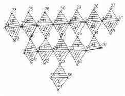
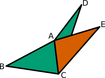       Example of a triplicate edge. Edge AC is used three times – by triangles ABC and ACD belonging to the green surface, and by triangle ACE belonging to the reddish surface.

       If a Triplicate line error message occurs during export, it means that three (or more) triangles are sharing an edge rather than just two, so the model doesn't form a simple closed surface. The error message includes the element numbers of the first two triangles involved. You can localize the problem by using the Plot command to display just those elements. For example, if the error message mentions elements 123 and 456, the following sequence of plot commands will display the two elements in relation to the rest of the model:

       1. p 5/grey (to display the whole model)
       2. p 1 6 123/-erase (to display a single type-6 shell element without erasing the previous plot)
       3. p 1 6 456/-erase (to display the second element)
       (You need to return to the Do? prompt before giving each of the p commands.)

       The Locate command can also then be used to determine the z coördinates and the approximate x and y coördinates of the nodes involved in the triangles, to help in locating the problem in Fie.

3. Run Gmsh.
   1. Use File ▶ Open to open the .geo file.
   2. Click on Mesh and then 3D.
   3. Wait for Gmsh to do the meshing and optimization.

      If you want to see the messages that are produced during processing, do Tools ► Message Console (or Ctrl-L). The contents of the message console can be saved by right-clicking within it and selecting Save Messages.

      If your mesh resolution is very high, Gmsh may take a long time to finish, and if there's something wrong with your model then Gmsh may not completely finish the job at all. If you then save the .msh file, you can then import it into Fad, but Fad may not find any of the tetrahedral elements that it is looking for, or they may not be optimized. Gmsh may also crash if your mesh is badly malformed. You may see a Segmentation fault error message if you run Gmsh from a terminal window under Linux (but not under MS Windows).

      If necessary, make your mesh resolution reasonable and correct any problems with your mesh, and then patiently wait for Gmsh to say that it has Done optimizing mesh before you try saving the results. If it says Done meshing 3D but never says Done optimizing mesh, there is probably something wrong with your model that is preventing Gmsh from generating a good mesh. Look at the message console as described above to see if there are warning or error messages.

      If there are error messages saying WARNING: Intersecting elements, then you need to figure out which elements are intersecting one another. The element numbers that it displays correspond to the element numbers in Fad. To find out where in your model the problem is, you can use Fad’s Select command followed by a Plot command to display a few elements around the offending elements. For example, if elements 55 and 85 are shown as intersecting, you might use this sequence of commands to display a few elements before and after each of those elements:
s none
s + 6 50,60
s + 6 80,90
p 3
      This works best if you don’t have too many elements.

      Gmsh will display a list of how many elements have quality values in the ranges 0.0 to 0.1, 0.1 to 0.2, …, 0.9 to 1.0. If that list is preceded by a warning message saying that some ill-shaped tets are still in the mesh, it means that those tetrahedra have quality values less than an arbitrary sliverLimit of 0.001. (See mesh/meshGRegionDelaunayInsertion.cpp, as of version 4.9.3, 2022 Jan 27.) That is indeed pretty bad if you want to use the mesh for finite-element analysis. You can use Fad’s p␣0/near and p␣/aspect to find the bad elements, as described above.

   4. Do File ▶ Export. Browse to the directory where your model files are and specify a filename. It is recommended that you append T to the file name to make it clear that the file contains a tetrahedral volume mesh rather than a surface mesh. Either explicitly include .msh at the end of the name, or select Mesh - Gmsh MSH (*.msh) as the desired file type. Click on OK.

      In the MSH Options dialogue that pops up, select Version 2 ASCII as the format. The boxes Save all elements and Save parametric coordinates should be unchecked. (The former doesn’t really matter but the latter does matter.) Click on OK.

   Alternatively, run Gmsh from the command line:
   gmsh filename.geo -3 -o filenameT.msh
   The vast amount of progress output can be suppressed by using > /dev/null or -v 2.
   The results are actually somewhat different when using the command line than when using the GUI, and I haven't yet figured out why.

4. Run Fad.
   1. Import (i command) the resulting .msh file into Fad. In the process, Fad will offer to retrieve boundary conditions, etc. from the .sap surface-model file that led to the .geo file that led in turn to the .msh file. The ability to retrieve boundary conditions and material properties from the original .sap surface file depends on the fact that Gmsh does not modify the original surface nodes or create new surface nodes, so Fad can establish a one-to-one correspondence between the original surface shell elements and the surface facets of the tetrahedral mesh produce by Gmsh.
   2. Use the Plot command with a plotting level of 3 (p␣3). A line should be displayed saying Nel13 = and a reasonable number of tetrahedral elements.
   3. Again, use p/near and p␣3/aspectratio to check for poor mesh quality.
   4. Use the Write command to save the tetrahedral model as a .sap file.
   5. If you need to create a model that contains multiple connected substructures, perform the above steps for each substructure. Then use the Join command to join them together. First join two of the substructures, then join a third substructure to the combination, and so on. At each stage, write out the combined model as a .sap file.
   6. Export (e command) the final model in the format required for further processing (e.g., as a .feb file for FEBio).

4. Element definitions